On Bayesian vs. Frequentist Learning

The dominant paradigm in modern machine learning is frequentist: we are given a batch of data, in the form of feature vectors and binary labels or real values, define some statistical model, and then define a loss function which is small when estimates given by this model are close to the target variables. The resulting model is then found by minimizing the loss averaged over data with respect to model parameters. This procedure subsumes model fitting in linear regression/classification, a Gaussian mixture model, or a deep network. The reason statisticians would consider this approach as frequentist, as opposed to Bayesian, is that information regarding the data distribution is not wielded in any way to inform how to select the model, and we typically have a uniform prior over distinct data points.

In this context, model selection is typically done based on domain expertise, rather than explicit metrics or structural properties of the data distribution. There are a few reasons for this:

1. One could argue that model selection (neural architecture specification, kernel hyper-parameters, etc.) is a heuristic attempt to encode information about the distribution;
2. Even if one could encode priors explicitly about the data distribution into the model training phase, for instance, to weight data points according to their importance, then it turns a standard numerical optimization procedure such as stochastic gradient method into a series of maximum a posteriori (MAP) updates, which may be computationally intractable.

Therefore, in order to employ information about arbitrary data distributions correctly in the modern model fitting paradigm, succinct representations of posterior distributions are required, as well as manners to make MAP updates efficient.

It’s well known that tracking only a posterior mean and covariance of the distribution of a hidden parameter may be done by a Kalman filter when the relationship between observations and hidden states are linear. This fact has led to recent efforts to use Kalman filters in ML. However, linearity is often a restrictive assumption, and much of modern advances in perception and speech recognition have been driven by nonlinear modeling. It therefore makes sense to integrate posterior distributions defined by nonlinear input-output relationships into model fitting.

When going beyond linear input-output models, tools such as Gaussian Processes (GPs) and Monte Carlo (MC) methods become of interest, which facilitate representing either Gaussian or arbitrary observation models, respectively. These tools are known to satisfy Bayesian analogues of the universal approximation properties of neural networks. Unfortunately, they suffer from an instance of the curse of dimensionality when the training sample size is large or samples arrive in a sequential fashion. In particular, computing the posterior mean and covariance of a Gaussian process has complexity cubic in the sample size. Similarly, computing the filtering density of a Monte Carlo method, a.k.a. a particle filter, also scales with the number of particles which must go to infinity to attain statistical consistency.

Therefore, in order to make Bayesian representations of posterior distributions applicable to the era of big data analytics, the computational challenges associated with large sample/particle sizes must be surmounted. In particular, we need finite memory approximations of GPs and MC methods that are near statistical consistency. While a number of memory-reduction techniques for both tools exist, their validation is predominately experimental [see Ch. 8 of the Rasmussen GP textbook], and a conceptual understanding of how to trade off memory and statistical consistency remains an active area of research.

In an upcoming companion blog post, we’ll give some perspective and discuss conceptual/practical tradeoffs of memory-reduction techniques of Bayesian methods.

Consensus Must Evolve for IoT/Autonomy

In the late 1990s, mathematicians and engineers became increasingly interested in trying to understand how spontaneous synchronicity occurs in nature. Specifically, there’s a book called Sync by Steven Strogatz (Applied Math, Cornell) which poetically describes how thousands of fireflies on the beaches of Thailand spontaneously blink in locked phase. Similar synchronicity occurs in schools of fish and flocks of birds as the group moves as a collective through only local coordination rules. The science of synchronicity gave rise to a provocative question for engineers in the 2000s: can we come up local coordination rules such that a collection of arbitrary agents (birds, fish, sensors, etc.) synchronize their behavior?

This question was probed, first in the math and physics community in the 1970s, in the context of Kuramoto oscillators and other mathematical models of electrical phenomena. Somewhat in parallel, control theorists John Tsitsiklis and Dimitri Bertsekas tried to connect these ideas to numerical optimization in the 1980s. Then, a famous series of papers beginning with “Coordination of groups of mobile autonomous agents using nearest neighbor rules” (Jadbabaie et al IEEE TAC 2003,) proposed a protocol in which each agent has a local state vector and updates its local state by computing a weighted local average of its neighbors’ states. Thereby, through only local communication, we can obtain globally emergent behavior: it can converge to a state that is common to all other agents, which  is the average of all agents’ individual states. This observation then yielded a burgeoning field of networked controls and distributed signal processing broadly referred to as consensus.

Numerous works built on top of the consensus protocol, primarily focusing on the case where agents not only seek to reach consensus but also minimize a convex function that is a sum of local functions available only to each agent. Famously, the paper “Distributed Subgradient Methods for Multi-Agent Optimization” (Nedich & Ozdaglar, IEEE TAC 2009) gave rise to the field of consensus optimization. In this work, the authors proposed a distributed version of gradient descent, that through only queries to agents’ local functions and weighted averaging with their neighbors, allows them to approximately reach the minimizer of a common global convex objective.

This algorithm was reinterpreted by the optimization community as a penalty method approximation of a constrained optimization problem, and therefore inferior to methods which can solve it exactly through use of Lagrange duality. The rest of the story of consensus optimization is about relaxing the conditions on the communications network that allows agents to exchange information, the technicalities regarding the objective to be minimized (from convexity to non-convexity, bounded gradients to unbounded gradients), and how to improve the learning rates by coming up with adaptations of acceleration and Newton’s method for decentralized settings.

Through all of these developments, consensus always presumes that agents reaching a common decision is the goal. However, we can easily envision technological applications in which this is not the case. Consider, for instance, an autonomous traffic network where sensory feeds on a car and a camera are both relevant to related inference tasks, but it is actively harmful (i.e., degrades local mean square error) for them to come up with identical statistical model parameters. This phenomenon holds more generally in heterogeneous networks such as ground and aerial robots, or IoT applications of smart devices in the home: the heterogeneity may be in agents’ observed data or the inference task they’re solving.

For these modern networked systems of intelligent smart devices, there is an open question of how to design the system such that the sum is more than the component parts. How does one agent exploit the relevant information of another, while ignoring irrelevant information? These questions motivate interesting questions that bridge decentralized optimization and game theory: when to communicate, what to communicate, and for which statistical learning tasks is this helpful? Two of my recent papers (listed below) provide a very small step in this direction from an optimization perspective; however, there is much more to be done that incorporates ideas from game theory.

A. Koppel, B. Sadler, and A. Ribeiro, “Proximity without Consensus in Online Multi-Agent Optimization,” in IEEE Trans. Signal Process., Mar. 2017.

H. Pradhan, A. S. Bedi, A. Koppel, and K. Rajawat, “Exact Decentralized Online Nonparametric Optimization,” in IEEE Global Conf. on Signals and Info. Processing (To appear), Anaheim, CA, Nov. 26-28, 2018.

 

Double Sampling: a Quirk of Reinforcement Learning

In supervised learning, we simply have a batch data in the form of training example, and fit a statistical model that maps features to target variables by minimizing a loss function. This loss function, for example, could represent the negative log-likelihood of a probabilistic model. Reinforcement learning is different because which statistical model parameters are chosen determine which data is observed next, and we’d like an optimal one starting from each different point. Intuitively, it sounds like this later setting would be more computationally intensive in terms of data required, and indeed this is the case.

In particular, a key characteristic which distinguishes optimization methods for supervised learning and reinforcement learning is the double sampling problem. Each step of a supervised learning procedure requires one data point, whereas each step of a reinforcement learning method requires two. In this blog post, we’ll rigorously explain  why this is the case. Before doing so, let’s first explain why in supervised learning we only need one training example per step.

In supervised learning, we try to minimize an objective which may be written as an expected value over a collection of random functions, each of which is parameterized by realizations of a random variable. Specifically, we care about the following stochastic program:

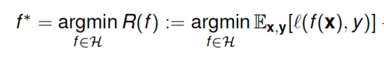
Here f is a statistical model that takes in feature vectors x and maps them to target variables y, 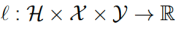  is a loss function that penalizes the difference between and quantifies the merit of a statistical model f evaluated at a particular sample point x.

To solve the above minimization when no closed form solution is available since the expectation cannot be evaluated (due to its dependence on infinitely many training examples), we require stochastic approximation. Thus, we perform gradient descent on the objective, but then approximate the gradient direction with an instantaneous unbiased estimate called the stochastic gradient. This is how maximum likelihood estimation, support vector machines, and many other searches for regression coefficients, are solved. It is not overstating things to say that the backbone of most modern supervised learning systems is a numerical stochastic optimization procedure called stochastic gradient method, which at each time implements the following

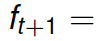
The validity of this approach crucially depends on unbiased estimates of the gradient being attainable via the stochastic gradient which requires only one training example to evaluate, i.e., there is only one sample  required to evaluate the stochastic gradient involving our current statistical model.

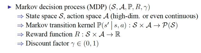
The landscape is different in reinforcement learning. We are faced with a more intricate question: not just how can we find a statistical model that maps features to targets, but how can we find a whole collection of models that map features to targets, such that when we condition on starting from an initial observation, we map to a initialization-specific target variable. Recall the basic setup of reinforcement learning from my previous post:

The goal in this setting is to formulate the average discounted accumulation of rewards when starting in a given state, which is called its value: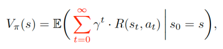and to choose the action sequence to maximize value. Since searching over infinite sequences is generally intractable, we typically parameterize the action sequence as a time-invariant (stationary) mapping called a policy:

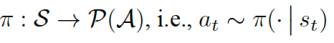
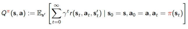
For further reference, when we condition the value function on a particular policy and initially chosen action, we call that the action-value (or Q) function, defined as:

There are two dominant approaches to finding an “optimal” policy, i.e. the one that makes the value as large as possible. One simply tries to do gradient ascent on the value function with respect to the policy, which is colloquially called “direct policy search.” The other, called approximate dynamic programming, employs ideas pioneered by Richard Bellman in the 50s. We’ll explain what each of these does, and why both approaches require at least two data points per update.

First, let’s focus on approximate dynamic programming, where we unravel the (action-)value function into its first term, the reward observed at the outset of the trajectory, and all subsequent rewards, which through some clever application of the properties of a Markov Process (such as the Kolmogorov-Chapman equation), yields the Bellman optimality equation. This expression, for a general continuous state and action space, is a fixed point equation that one must satisfy for each initial point in the space, i.e., we would like to find Q functions that satisfy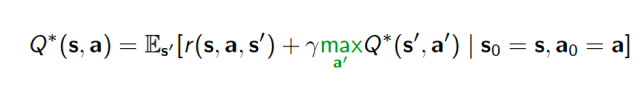for all s and a. The above expression is called the Bellman optimality equation (Bellman ’57). Now, we can define the temporal difference (Sutton ’98) as:

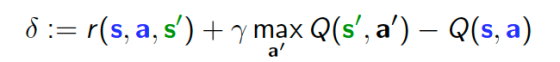
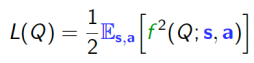
which is how far the Q function is from satisfying the Bellman optimality equation for a given state-action-state pair. We can define the average deviation from optimality when starting from a given s and a as:

If we define an ergodic distribution over the state and action spaces, that is, a distribution for which visiting any state-action pair occurs with positive probability, we can transform the above stochastic fixed point problem into an optimization problem where the decision variable is the Q function. Moreover, the universal quantifier regarding initialization may be re-expressed as an additional expectation over all starting points of the Markov Decision Process trajectory. Therefore searching for the optimal (action-)value function involves an optimization problem involving nested dependent expectations.

This observation was famously explained by Sutton in 2009 (“A Convergent O ( n ) Algorithm for Off-policy Temporal-difference Learning with Linear Function Approximation”).

The presence of the inner and outer expectation mean that computing the functional stochastic gradient of the above loss will depend on an additional inner expectation that must itself be estimated by a second process. Therein lies the origins of the double sampling problem in approximate dynamic programming (ADP). The fact that the nested expectations must be overcome while ensuring the Q function parameterization remains stable and also moderate memory is a key challenge of ADP. The most convincing ways of dealing with this in ADP is to either connect ADP with stochastic compositional optimization and formulate a time-average recursive estimator or a sample average approximation of some the inner expectation to plug into the outer one, as in some of my recent works (“Policy Evaluation in Continuous MDPs with Efficient Kernelized Gradient Temporal Difference” and “Nonparametric stochastic compositional gradient descent for q-learning in continuous Markov decision problems”) or a clever use of the Fenchel dual to reformulate the Bellman optimality equation as a saddle problem (“Stochastic Dual Dynamic Programming (SDDP) ” and “SBEED: Convergent Reinforcement Learning with Nonlinear Function Approximation”).

The other dominant approach to reinforcement learning, as previously mentioned, is direct policy search, of which the canonical method is policy gradient ascent (“Policy Gradient Methods for Reinforcement Learning with Function Approximation”). It sounds intricate, but really, it’s gradient ascent on the value function defined above, while using the log trick and some other properties of the Markov process. In particular, if we parameterize the policy:  and define the value function above as J. Then the Policy Gradient Theorem states that:

where the expectation is taken over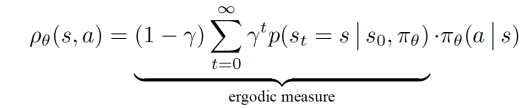 

that is parameterized by the policy parameters. Policy gradient ascent simply executes the update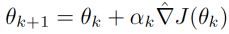 but the validity of this update crucially requires the gradient estimate here to be an unbiased estimate of the aforementioned expanded expression.

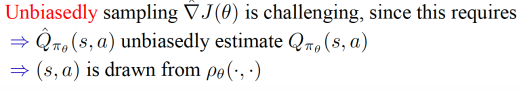
In particular, the Q function in the policy gradient is itself another expectation (see the definition of Q from the ADP discussion) but taken over a distribution that depends on the policy parameters. Hence, from a completely different perspective than Bellman’s dynamic programming equations, we have arrived at the fact that direct policy search runs into double sampling.

Many policy search methods attempt to overcome this setting by operating in a hybrid scenario where the Q function may be estimated in a batch fashion called episodic reinforcement learning, or simply plug in a mini-batch estimate for Q into the infinite horizon case and hope for the best. But in general, unbiasedly estimating the Q function in the infinite horizon case remains a challenging problem since the expectation upon which the Q function depends is parameterized by the policy parameters.

The “Jungle” of Reinforcement Learning: Policy Evaluation versus Policy Learning when On and Off Policy

Reinforcement learning is a mathematical framework for data-driven control, and defines a situation in which an autonomous agent seeks to learn to take actions based on rewards it observes that come from the environment it traverses. In particular, its a formalism for trying to teach a learning agent to try to follow temporally related incentives, like a trail of bread crumbs.

In light of the smashing success of AlphaGo during the summer of 2016, reinforcement learning has received increasing attention from disparate academic communities such as machine learning, artificial intelligence, control systems, operations research, and applied mathematics. However, the research communities view the same problem fairly differently, and as a result there is a noticeable gap between methods for reinforcement learning which are theoretically sound versus practically useful. Compounding this “practicality gap” is the imprecise language which is used to describe practical approaches reinforcement learning, e.g., when describing “off policy policy evaluation,” what do we really mean, mathematically? The purpose of this blog post is to clarify the taxonomy of different problems in the field, and what are the challenges one must face when in each setting. Before doing so, I’ll review a few basic concepts so we are on the same page.

Reinforcement learning is defined by a setting in which an autonomous agent moves through some environment (state space), which is typically a compact subset of Euclidean space. At some time, the agent takes an action which belongs to some other compact Euclidean subset, and then the agent moves to a new state. The way this transition happens is random, but is dependent on the previous state and action taken. Then a reward is revealed by the environment, which informs us of how good the action was. 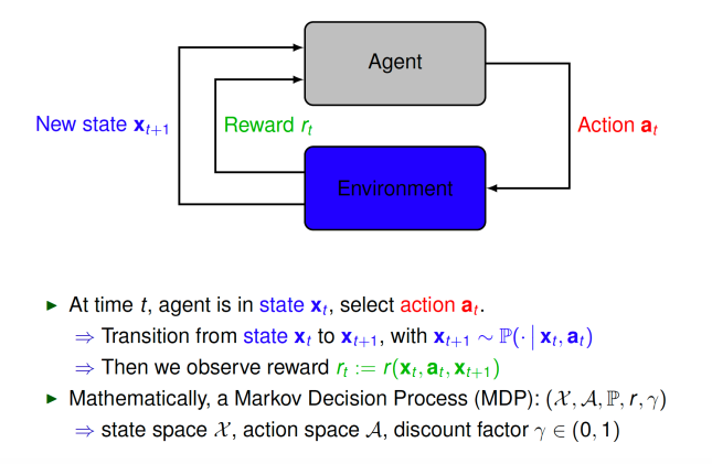See the cartoon below, taken from one of my recent presentations:Here I am discussing the most general case where state and action spaces are continuous, which is in contrast to the context in which classical dynamic programming theory was developed. The average accumulation of rewards when starting in a given state is called its value: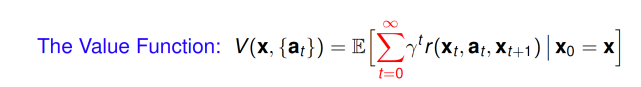The goal in reinforcement learning is to chose the action sequence so as to accumulate the most rewards on average. 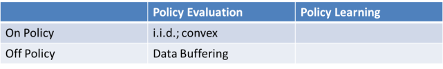Thus, our target is always to find the action sequence which gives us the most value: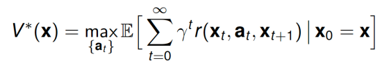Now that we are all on the same page, we can talk about what are the difficulties of actually determining the optimal policy. I’ll organize the discussion according to the following table:

1. Top left: To actually optimize the value function with respect to our action sequence, we need to first have access to the value function, i.e., the above equation requires the one before it as a prerequisite. This is can be stated intuitively as policy improvement cannot happen without first knowing how to evaluate a policy. But to evaluate a policy, the agent must move around its environment according to a fixed policy for awhile, meaning that a lot of behavior occurs that’s not actually valuable. This setting of learning the value associated with a fixed policy is called policy evaluation. This may only be guaranteed to converge when the policy (in the form of state-action-reward triples) we evaluate is associated with value function we are learning, i.e., on-policy. On the positive side, it is possible to find stochastic approximation algorithms that converge almost surely and determine the value function for a fixed policy. This fact fundamentally hinges on the fact that the state-action-reward triples are independent and identically distributed (i.i.d.), and the fact that it’s possible to reformulate this task as a stochastic convex optimization problem.
2. Bottom left: When trying to determine the value function when the data does not follow the policy we are evaluating, we are in murky territory. People keep around “training data sets” consisting of state-action-reward triples and keep running their value function estimation scheme until “convergence” but it is not at all clear that convergence is possible, since any stochastic descent direction or fixed point iteration will necessarily be biased. This is because when we compute expectations over data, we are computing expectations over data that is different from that which defines the value function! Put another way, we lose the crucial i.i.d. property of our data. A lot of heuristics and complicated tricks are used to circumvent this issue, such as importance sampling, biased replay buffers, probabilistic exploration schemes, encoding Bayesian priors on the value function, etc. But we lack a good theoretical understanding of these tools in terms of how they actually help or hurt us in determining which actions have the most value.

   To summarize, when we are learning the value function associated with the actions the agent actually follows, this is on-policy policy evaluation. When we try to learn the value function not associated with the actions chosen, we’re in the murky territory of stochastic optimization with an expectation over data not seen.

3. Now, let’s move to the second column, still in the second row (bottom right). Policy learning when off policy is the province of classical Q learning and TD Backgammon. The idea here is that the agent, by taking random actions, and then learning their associated value, will eventually learn the optimal value function. However, a fundamental difference between this setting and the first column is that all formulations of policy learning eventually boil down to a non-convex optimization problem, with the exception of stochastic fixed point iteration (classical TD(0)-style Q learning), but it’s an open question whether fixed point iteration is stable under function approximation. Function approximation, unfortunately, is required when operating in continuous spaces. This non-convexity, rather than being an artifact of the way we define a nonlinear statistical model, as in deep learning, is instead intrinsic to the problem formulation, as it is for the Traveling Salesman Problem or Cauchy-Schwarz Quadratic Mutual Information.
   • Non-convexity in policy learning is a challenging problem because even if we design a method that converges with probability 1, it could converge to an arbitrarily bad stationary point. To avoid this, people try to tamper with the random i.i.d. nature of the exploratory policy used in off-policy learning by biasing it towards states that are “more likely” to yield high rewards. But doing so can break the stochastic contraction/descent properties of the learning method. This is one example of the explore-exploit tradeoff. To learn a good policy, we have to randomly fully explore the space. But doing so could take a very long time during which we get very little reward. So instead we bias the action distribution. But this bias can cause the learning process to diverge.
4. Lastly, the top-right corner, policy learning when on-policy, is best equipped to mitigate problems associated with the explore-exploit tradeoff. However, doing so comes at the cost of data now exhibiting temporal dependence. That is, now the learning process must address the fact that it is observing correlated time-series data, a setting under which theoretical understanding of stochastic optimization methods mostly breaks down. Some efforts to understand how to do supervised learning from time-series in very specialized settings, when one limits the amount how non-i.i.d. the data may be, have been developed. But serious mathematical sophistication required to understand this setting, and the analysis pretty much says: we can’t change the policy too quickly while learning, otherwise the value function never converges. This data distribution difficulty compounds the difficulties of non-convexity and/or stochastic fixed point iteration with function approximation that are present in the off-policy setting. However, somewhat remarkably, experimentally, on-policy policy learning can obtain very good results…if it does not diverge.

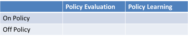
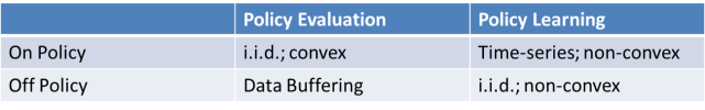To sum up the above discussion, let’s now look at the filled in table:The takeaway from this blog post is that (1) we would like to overcome non-convexity in policy learning. The only way to do this is with stochastic fixed point iteration, but we don’t know how to make this work with function approximation, which is required for continuous spaces; (2) non-convexity is a major contributor to the phenomenon called the explore-exploit tradeoff, for if we had convexity, through random exploration alone we would always eventually find the best policy; (3) on-policy policy learning can experimentally obtain very good results, but theoretically it requires treating trajectories through the space as time-series, a setting for which most understanding of statistical learning methods breaks down; and (4) hacks such as biasing action selection towards states that yield higher reward (greedy actions) can help us mitigate the explore-exploit tradeoff but we possibly do so at the cost of our learning process diverging.

A Digression on Narrow and General Artificial Intelligence

In my last blog post, I went on a diatribe on how far current technology is from anything resembling the machines of Blade Runner or Terminator. Admittedly, some of this diatribe was fueled by disdain for those who make strong declarations about topics for which they are unqualified. But this diatribe was equally fueled by the scientific limits of what is currently possible. Since evidence is more convincing than disdain, I’ve chosen to focus on providing some as the focus of a follow up blog post.

Specifically, I’ll focus on what in the lore we call Narrow Artificial Intelligence (e.g., an iPhone or the software equipped in most modern automobiles) and General Artificial Intelligence (think HAL from 2001: A Space Odyssey), and the technical challenges of transforming the former into the later. What is it that makes HAL so much harder to program than Siri or your learning thermostat? That’s the scope of this discussion. Let’s focus on the broad contours of how speech recognition systems work, due to their increasing ubiquity among consumer electronics, and the fact that most intelligent systems begin from a similar pipeline.

1. First we need to accumulate training data, possibly on the order of billions of sample points.
   • This is affordable for speech systems. For designing management strategies or robotic controllers, it is definitely not.
2. Now we take all this data and try to find a more illuminating representation of it (say, using clustering, principle component analysis (PCA), or a multi-layer variant of PCA called an autoencoder). To complete this step, typically one must analyze the sample covariance matrix of the data and solve some numerical optimization problem involving it. Alternatives to PCA/autoencoders include taking all data which is similar according to some distance and putting it in the same bag (k-means/nearest neighbor clustering). This is what Netflix used to do for recommending similar movies to what you’ve watched recently.
   • This signal representation step is called unsupervised learning, and is really about adopting the right “perspective” of the data domain. Think of this as your underlying worldview. It’s a lot easier to make decisions if you first learn to decide what are the defining characteristics of a given context.
3. Now we need to build the statistical decision maker, i,.e., the supervised learning step. This step was briefly discussed in my last post, and follows ideas dating back to Sir R. A. Fischer. Now that we have designed our data representation (step 1), we need to decide how to map data to decisions. This happens by first making sure that all of our data has labels (apple or orange, happy or sad), or more generically target variables. Then we postulate that our decision function takes a specific form, say, a mixture of Gaussians centered at our input data (kernel methods) or a deep convolutional network. Then, we specify a merit criterion which is small when our decision function maps data to be close to its target variable, and we try to choose our decisions such that this loss function is minimized on average over all data.
   • Actually solving this minimization problem and it’s interplay with the choice of the functional form of our decision function is challenging. As a result, optimization for supervised learning is a very active area of research among scientists spanning the fields of statistics, machine learning, signal processing, controls, operations research, and applied mathematics. I dedicate much of my professional time to this challenge. Typically we build upon iterative numerical schemes such as gradient descent or Newton’s method, and their stochastic variants which operate on small subsets of data per step.

Now that we have outlined what is the standard pipeline for learning systems as they exist today, which people intuitively think of as intelligent, we can begin to broach why this intelligence is Narrow, not General. All of the aforementioned machinery is used to build a decision system that spits out an answer of the form apple or orange, or a sequence of apples versus a sequence of oranges. This works well enough for simple tasks like building up a text response to a spoke statement when we combine it in a piecemeal fashion with other similarly designed statistically generated decisions. However, fundamental challenges remain when trying to “teach” a system higher level knowledge as compared with simple one-layer Q&A:

1. We don’t know how to combine decision functions (estimators) in a mathematically stable/convergent way. I can teach my learning system to recognize a cat exceptionally well from a bunch of images of cat and no cat. However, we know that cats belong to a phylogenetic tree, which begins at kingdom and proceeds to phylum, …, genus, species. Each of these classifications must be done at a branch of the tree with a distinct decision function that should be daisy-chained from its root to its leaf.  We have NO IDEA how to do this in a way that makes sense from the perspective of mathematical statistics. Some efforts in finance and operations research on two-stage (and multi-stage) stochastic programming have tried to answer this question but can only be addressed for very restrictive cases. But, without devolving into a detailed discussion of multi-stage stochastic programming, this bottleneck exists because of fundamental limits of our current optimization algorithms, which may be insurmountable. The way around these limits that has appeared in practical systems like an Autopilot or Siri is to “hand-tune” when estimators fit into more complicated systems, but this only works well when each component of the system is well-understood, as in classical aerospace applications. For general data-driven learning systems, this is far from true.
2. Suppose for the sake of argument that issue 1 is solved, and that we can have an agent learn a hierarchical decision system. Then we are faced with how to encode learning higher-level behavior like a principle or a value into statistical learning systems. Here I mean principle or value in the common understanding, as in “our society values ambition and vision.” One possible solution would be to encode an intangible quality like virtue or bravery or honesty mathematically as some sort of constraint on the way the system makes decisions and augmenting the above learning procedures to address these constraints. But then engineers will find themselves in the murky business of mathematically encoding human emotions and principles, which in my humble opinion is impossible. While psychologists have endeavored to find quantitative measures of human emotions, there’s still a huge gap between “we observed something in a controlled lab experiment” and “this is how a certain human behavioral phenomenon occurs in general.” And therefore, most of the quantitative models developed by psychologists cannot be applied to develop learning systems as if they are just another engineering tool.
3. Once the preceding two problems are taken care of (which may take decades), we are still faced with the open-ended question: if we string together enough binary classifications or regressions together, does higher-level reasoning emerge? In essence, what I am asking is, do most questions of “why?” or “how?” break down into a string of “what?” or “how much?” questions? The answer most people would give is sometimes yes, sometimes no. The answer to “why did the cookies burn?” can be easily addressed with a sequence of “what” questions, but the answer to “why is faith in democracy waning globally?” is much less straightforward. We are arbitrarily far from having a machine learn from experience how to answer the later question, and this is what I claim produces the chasm between Narrow AI and General AI.

I should caveat the preceding discussion by the fact that there are many ways of approaching the construction of machine intelligence from data and experience. I have chosen to adopt a perspective based on mathematical statistics, optimization, and machine learning, since these fields are driving forces behind recent advances at Google, Microsoft, Facebook, etc. The perspective/criticism from members of other research communities, especially computer vision, natural language processing, linguistics, and psychology, would help to qualify the above discussion, and hopefully spawn the development of new ideas to advance the state of machine understanding.

The Chasm between Artificial Intelligence in the Public Imagination and Technology Today

The prognostications of Silicon Valley moguls such as Elon Musk, Peter Thiel, and company would have you believe we are standing on the edge of an artificial intelligence apocalypse, with smart machines coming to eat everyone’s lunch and undermine the viability of the economy as it functions today. This anxiety is exacerbated by recent troubling news of the way Big Tech is manipulating things we hold dear, such as local organic dispensers or civil democratic discourse. Combined with a steady diet of dystopian motion picture depictions of intelligent machines such as 2001: A Space Odyssey, Bladerunner, Her, Ex Machina, The Terminator, AI, Alien: Covenant, and so on, one may come away with the impression that the magnates of Big Tech are correct: the future of humanity is slipping out of the grasp of humans and into that of some nameless,  faceless Machine Learning systems.

I’ve spent the past several years during graduate school and onward becoming intimately familiar with the mathematical underpinnings of learning theory and how it can be used to design autonomous learning systems. What I can tell you is that we are exceptionally far from designing anything resembling intelligence in the popular usage of the word. Today’s learning machines can successfully learn from their sensory feeds to address rudimentary questions such as “am I looking at an apple?” with a high degree of accuracy. This is called supervised learning, or statistical inference, and dates back to Sir R. A. Fischer in 1917. The key difference between then and now is increased data availability and computing infrastructure, but the bones of how the learning occurs is nearly as basic as it was in 1917.

Within the next five to ten years will be able to reliably and from streaming information have a learning system, not just perform object recognition (“is that an apple”?), but learn to autonomously navigate its environment through past trial and error experiences. To be specific, we will be able to teach an autonomous agent to ask the right questions that lead it to find the apple. This is called reinforcement learning, and has been around at least since Richard Bellman in 1954, but the framework has gained salience more recently, again due to increases in computing power and data availability. The folks at Google DeepMind, among others, are hard at work on making this a reality for simple videogames, and from that we will be able to extrapolate the techniques to problems faced by robotic systems.

But what no engineered combination of supervised or reinforcement learning systems can tackle is how to mathematically formulate the meaning of higher level questions or abstract notions. There is an insurmountable barrier between “how should you steer to the apple?” and “what is the meaning or purpose of an apple?” that makes it beyond the realm of engineered systems. Workarounds based on regurgitating information from Wikipedia or Google ignore the issue of how a machine should actually form a representation of higher-level knowledge based on what it’s trying to do. There really is nothing that both makes mathematical sense and captures the way abstract concepts actually can define the real world and our experience of it.

I would like to go out on a limb at this point and claim that we will never be able to assign a numerical value to intangible concepts like trust, friendship, creativity, and so on. Without a formal theory of how learning systems should process and understand abstract concepts, no engineered systems will do so. We may see exceptions within our lifetime, but these will not go beyond a “special sauce” cobbling together of different features to dupe us into believing we are observing intelligence when we really are not. Siri and Alexa don’t understand you. Not really. They just built up an intricate predictive statistical model of your speech patterns and browsing habits. But there is no higher level understanding.

Equipped with this understanding of the limitations of the artificial intelligence of our imagination, we can shift focus to how technology is currently evolving. Products like the iPhone, HomePod, Echo, XBox One, etc., promise consumers intelligent companionship that can understand when important events are upcoming in their lives and help them find recipes in real time for things they are cooking. For all sorts of rudimentary tasks like recounting information from the web or inside your smartphone apps, they are well-equipped to do so. But this impressive functionality breaks down when you replace basic informational questions with ones that require any sort of creativity and synthesis. For higher-level knowledge, there’s nothing more than regurgitating Wikipedia.

These products are a lot more rudimentary than the marketing campaigns for Amazon Echo, HomePod, etc. would have you believe. Big Tech has a vested interest in convincing the public that autonomous learning systems are much more advanced than they are, so that in five to ten years we are more likely to buy into the rush towards autonomous cars. Automobile companies are pouring billions of dollars into the development of AI for autonomous driving, ignoring the sheer number of higher-level questions that are required during our daily driving experience, such as how to provide an intuitive and adaptive response to the behavior of a cyclist in a neighboring lane on the road. This should give us cause for concern.

More pernicious than a few malfunctioning fancy cars are the long-term economic effects that industrial automation has wrought on the working classes of Western countries. Automation has been so effective because it allows autonomous systems to operate only within the realm of low-level questions and repetitive mechanical tasks, for which identifying the apple and navigating to it are enough.  As countries have automated factories, warehouses, cashiers, and other components of retail, decent working people have watched their livelihoods evaporate. We cannot ask companies to reduce efficiency and incur greater operating costs just due to our bleeding hearts. The task we are faced with is how to redirect working people to tasks that are well-suited to their skill set, and too challenging for industrial engineers to automate. The AI Apocalypse may not be coming, but the bifurcation of advanced industrialized economies is already here.